elm <-function(X, y, n_hidden=NULL, active_fun=tanh) {# X: an N observations x p features matrix# y: the target# n_hidden: the number of hidden nodes# active_fun: activation function pp1 =ncol(X) +1 w0 =matrix(rnorm(pp1*n_hidden), pp1, n_hidden) # random weights h =active_fun(cbind(1, scale(X)) %*% w0) # compute hidden layer B = MASS::ginv(h) %*% y # find weights for hidden layer fit = h %*% B # fitted valueslist(fit= fit, loss=crossprod(fit - y), B=B, w0=w0)}# one variable, complex function -------------------------------------------library(tidyverse); library(mgcv)
── Attaching packages ─────────────────────────────────────── tidyverse 1.3.2 ──
✔ ggplot2 3.4.1     ✔ purrr   1.0.1
✔ tibble  3.1.8     ✔ dplyr   1.1.0
✔ tidyr   1.3.0     ✔ stringr 1.5.0
✔ readr   2.1.3     ✔ forcats 1.0.0
── Conflicts ────────────────────────────────────────── tidyverse_conflicts() ──
✖ dplyr::filter() masks stats::filter()
✖ dplyr::lag()    masks stats::lag()
Le chargement a nécessité le package : nlme


Attachement du package : 'nlme'


L'objet suivant est masqué depuis 'package:dplyr':

    collapse


This is mgcv 1.8-41. For overview type 'help("mgcv-package")'.
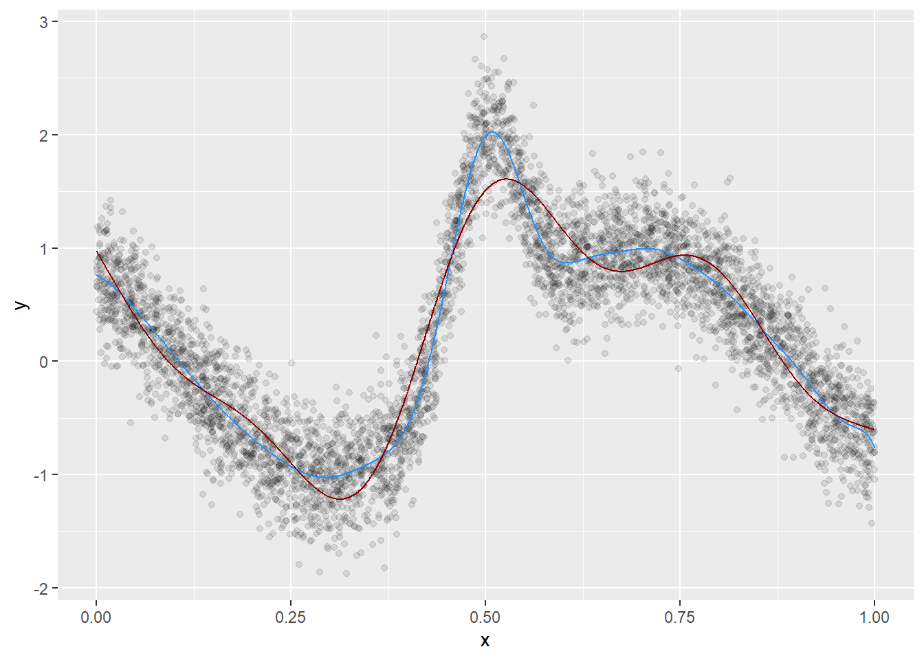
set.seed(123)n =5000x =runif(n)# x = rnorm(n)mu =sin(2*(4*x-2)) +2*exp(-(16^2)*((x-.5)^2))y =rnorm(n, mu, .3)# qplot(x, y)d =data.frame(x,y) X_ =as.matrix(x, ncol=1)test =elm(X_, y, n_hidden=100)str(test)
List of 4
 $ fit : num [1:5000, 1] -1.0239 0.7311 -0.413 0.0806 -0.4112 ...
 $ loss: num [1, 1] 442
 $ B   : num [1:100, 1] 217 -608 1408 -1433 -4575 ...
 $ w0  : num [1:2, 1:100] 0.35 0.814 -0.517 -2.692 -1.097 ...
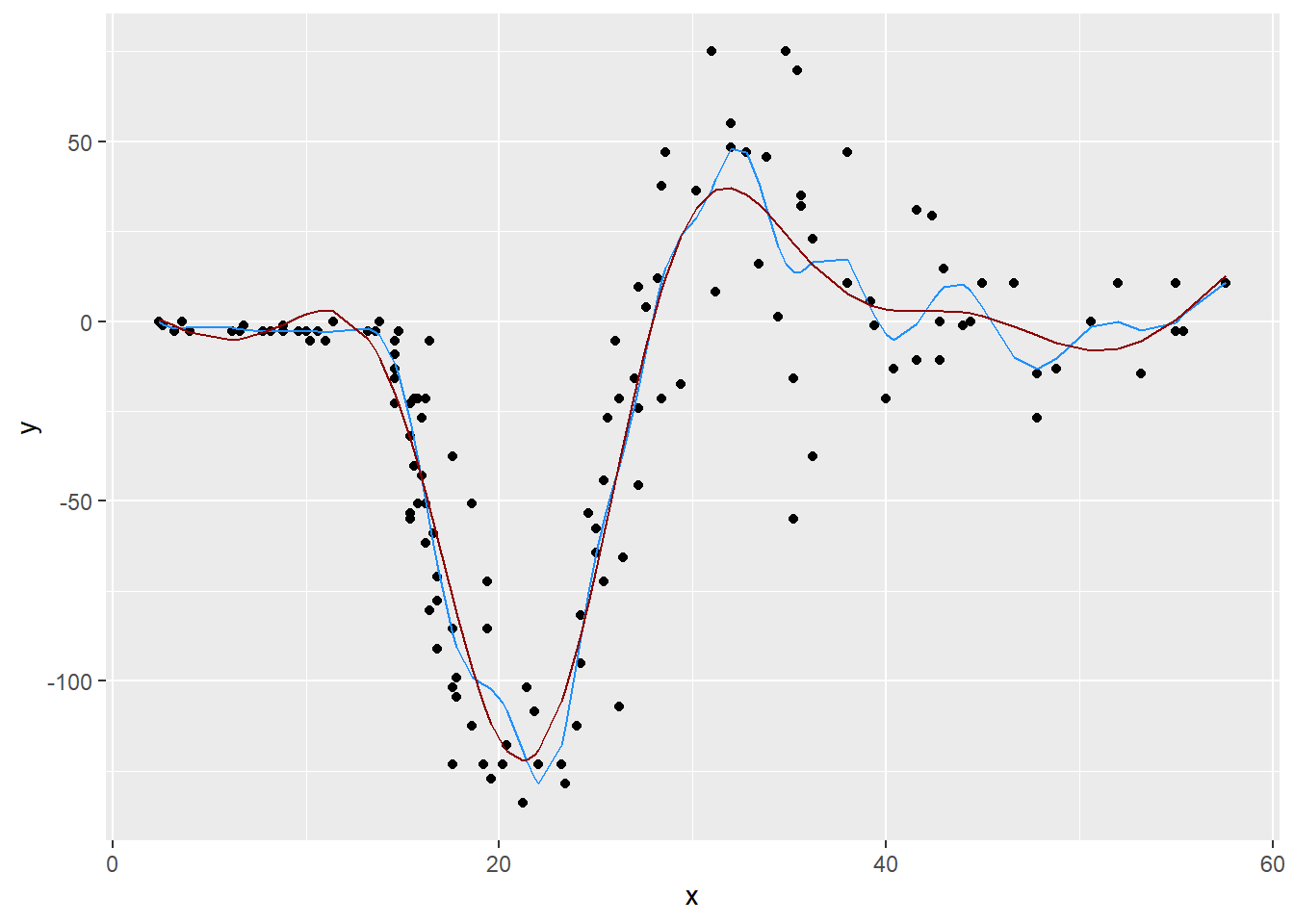
Gu & Wahba 4 term additive model, correlated predictors
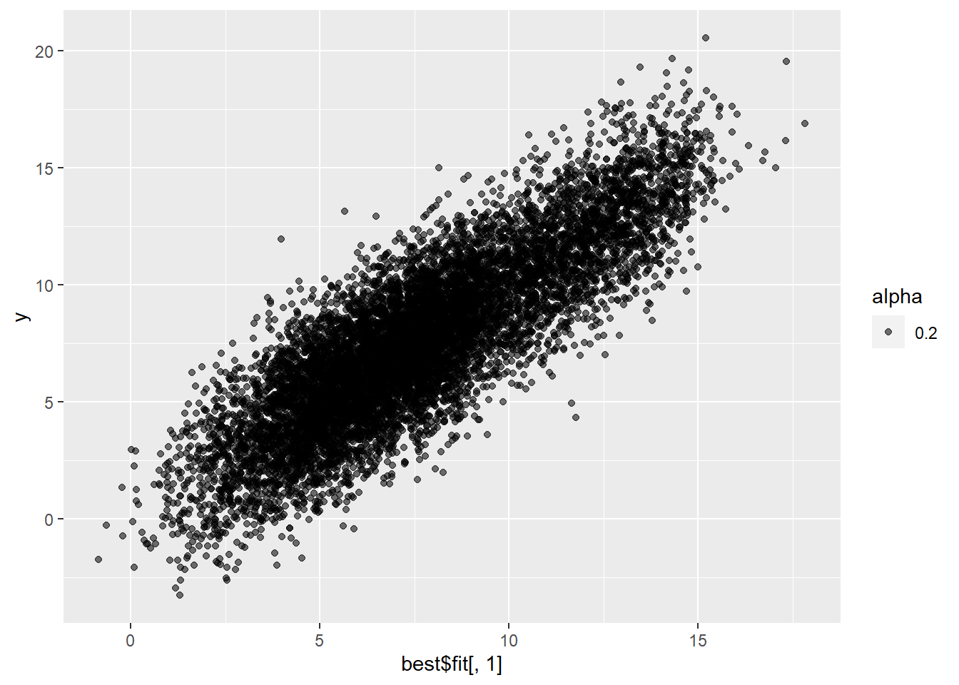
X_ =as.matrix(d[,2:5])y = d[,1]n_nodes =c(10, 25, 100, 250, 500, 1000)test =lapply(n_nodes, function(n) elm(X_, y, n_hidden=n)) # this will take a few secondsfinal_n =which.min(sapply(test, function(x) x$loss))best = test[[final_n]]# str(best)qplot(best$fit[,1], y, alpha=.2)
Method: GCV   Optimizer: magic
Smoothing parameter selection converged after 15 iterations.
The RMS GCV score gradient at convergence was 9.309879e-07 .
The Hessian was positive definite.
Model rank =  37 / 37

Basis dimension (k) checking results. Low p-value (k-index<1) may
indicate that k is too low, especially if edf is close to k'.

        k'  edf k-index p-value
s(x0) 9.00 4.71    1.00    0.48
s(x1) 9.00 4.89    1.00    0.35
s(x2) 9.00 8.96    0.99    0.20
s(x3) 9.00 1.00    1.00    0.47
summary(gam_comparison)$r.sq
[1] 0.6952978
test_data0 =gamSim(eg=7) # default n = 400
Gu & Wahba 4 term additive model, correlated predictors
test_data =cbind(1, scale(test_data0[,2:5]))elm_prediction =tanh(test_data %*% best$w0) %*% best$B # remember to use your specific activation function heregam_prediction =predict(gam_comparison, newdata=test_data0)cor(data.frame(elm_prediction, gam_prediction), test_data0$y)^2