Cubic Splines

library(tidyverse) # for processing and plotting

── Attaching packages ─────────────────────────────────────── tidyverse 1.3.2 ──
✔ ggplot2 3.4.1     ✔ purrr   1.0.1
✔ tibble  3.1.8     ✔ dplyr   1.1.0
✔ tidyr   1.3.0     ✔ stringr 1.5.0
✔ readr   2.1.3     ✔ forcats 1.0.0
── Conflicts ────────────────────────────────────────── tidyverse_conflicts() ──
✖ dplyr::filter() masks stats::filter()
✖ dplyr::lag()    masks stats::lag()

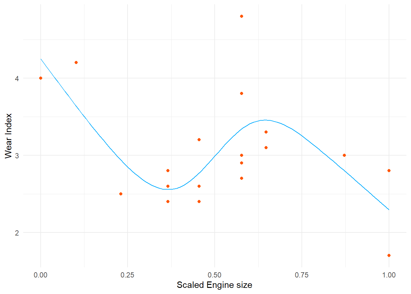
#' # Create the data
size = c(1.42,1.58,1.78,1.99,1.99,1.99,2.13,2.13,2.13,
         2.32,2.32,2.32,2.32,2.32,2.43,2.43,2.78,2.98,2.98)

wear = c(4.0,4.2,2.5,2.6,2.8,2.4,3.2,2.4,2.6,4.8,2.9,
         3.8,3.0,2.7,3.1,3.3,3.0,2.8,1.7)

x = size - min(size)
x = x / max(x)
d = data.frame(wear, x)

#' Cubic spline function
rk <- function(x, z) {
  ((z-0.5)^2 - 1/12) * ((x-0.5)^2 - 1/12)/4 -
    ((abs(x-z)-0.5)^4 - (abs(x-z)-0.5)^2/2 + 7/240) / 24
}

#' Generate the model matrix.
splX <- function(x, knots) {
  q = length(knots) + 2                # number of parameters
  n = length(x)                        # number of observations
  X = matrix(1, n, q)                  # initialized model matrix
  X[ ,2]   = x                         # set second column to x
  X[ ,3:q] = outer(x, knots, FUN = rk) # remaining to cubic spline basis
  X
}

splS <- function(knots) {
  q = length(knots) + 2
  S = matrix(0, q, q)                         # initialize matrix
  S[3:q, 3:q] = outer(knots, knots, FUN = rk) # fill in non-zero part
  S
}

#' Matrix square root function. Note that there are various packages with their own.
matSqrt <- function(S) {
  d  = eigen(S, symmetric = T)
  rS = d$vectors %*% diag(d$values^.5) %*% t(d$vectors)
  rS
}

#' Penalized fitting function.
prsFit <- function(y, x, knots, lambda) {
  q  = length(knots) + 2    # dimension of basis
  n  = length(x)            # number of observations
  Xa = rbind(splX(x, knots), matSqrt(splS(knots))*sqrt(lambda)) # augmented model matrix
  y[(n+1):(n+q)] = 0        # augment the data vector
  
  lm(y ~ Xa - 1) # fit and return penalized regression spline
}



#' # Example 1


#' Unpenalized
#' 
knots = 1:4/5
X = splX(x, knots)      # generate model matrix
mod1 = lm(wear ~ X - 1) # fit model

xp = 0:100/100 # x values for prediction
Xp = splX(xp, knots) # prediction matrix


#' Visualize

ggplot(aes(x = x, y = wear), data = data.frame(x, wear)) +
  geom_point(color = "#FF5500") +
  geom_line(aes(x = xp, y = Xp %*% coef(mod1)),
            data = data.frame(xp, Xp),
            color = "#00AAFF") +
  labs(x = 'Scaled Engine size', y  = 'Wear Index') +
  theme_minimal()

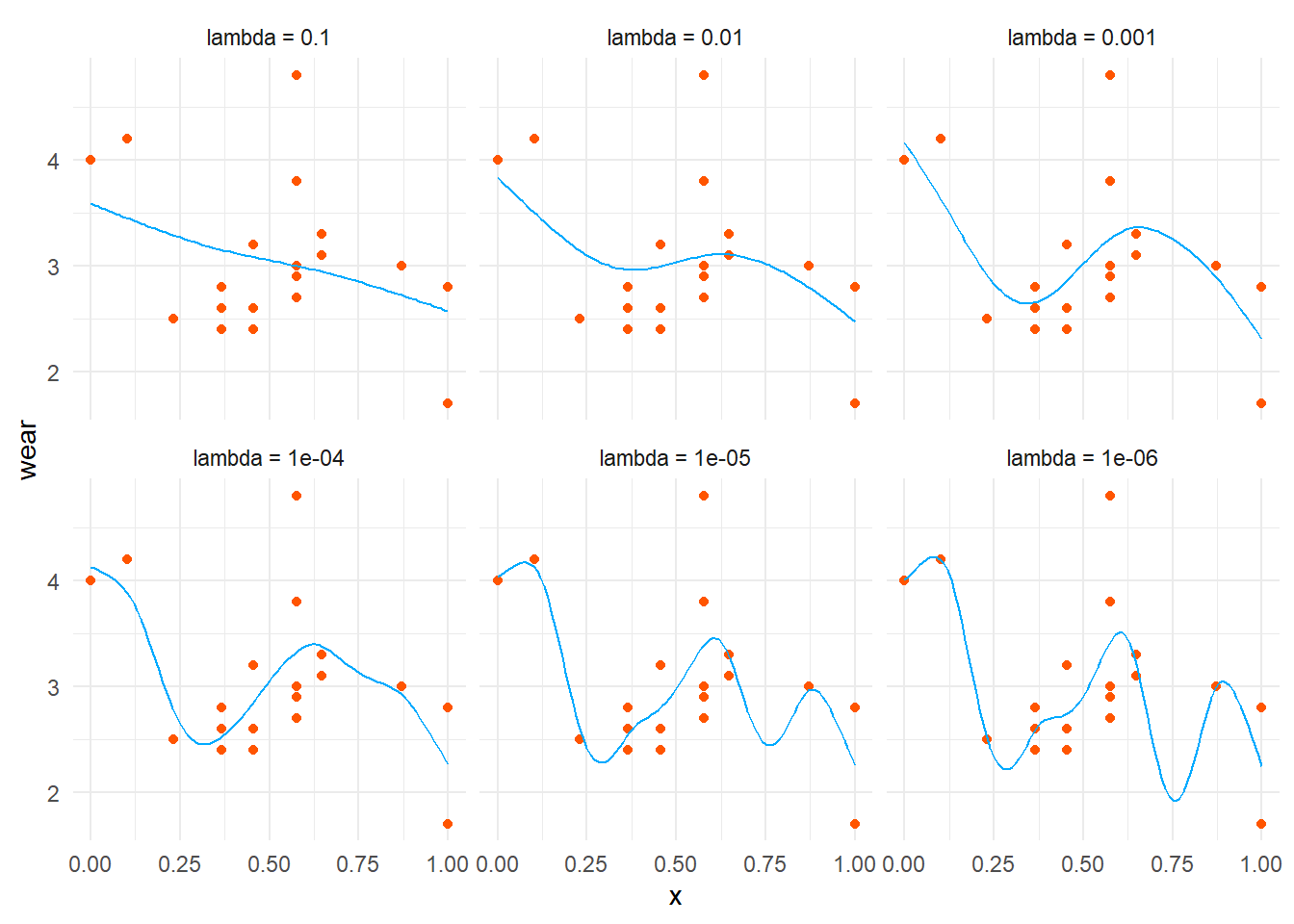
#' # Example 2


# Add penalty lambda
knots = 1:7/8
d2 = data.frame(x = xp)

for (i in c(.1, .01, .001, .0001, .00001, .000001)){
  # fit penalized regression
  mod2 = prsFit(
    y = wear,
    x = x,
    knots = knots,
    lambda = i
  ) 
  # spline choosing lambda
  Xp = splX(xp, knots) # matrix to map parameters to fitted values at xp
  LP = Xp %*% coef(mod2)
  d2[, paste0('lambda = ', i)] = LP[, 1]
}

#' Examine
# head(d2)

#' Visualize via ggplot
d3 = d2 %>%
  pivot_longer(cols = -x,
               names_to  = 'lambda',
               values_to = 'value') %>% 
  mutate(lambda = fct_inorder(lambda))

ggplot(d3) +
  geom_point(aes(x = x, y = wear), col = '#FF5500', data = d) +
  geom_line(aes(x = x, y = value), col = "#00AAFF") +
  facet_wrap(~lambda) +
  theme_minimal()